If you’ve been a long time follower of our blog, you’ll remember the handful of guest posts about my PhD research. So far results have been focused on a few key species (mountain laurel, huckleberry, and hay-scented fern), and whether environmental conditions (like soil chemistry and topography) explain whether any of these species are present at a site (occupancy probability).
What about groups of species? We know that forests are complicated places with organisms interacting with each other and their environment. There are countless interactions that occur in ecological communities, so how in the world do we separate those effects?
Experimental manipulation is one approach, and I’ll talk more about the results of my liming, herbiciding, and fencing treatments in a later post. Another method is to use multivariate statistics. While this may sound complicated, it is actually one of the easiest ways to explore habitat patterns across sampling locations.
With some help, I collected full inventories of vegetation data (seedlings, little green stuff, and overstory trees) across 261 subplots at 24 sites. There’s no way my little human brain can recognize vegetation patterns across all of these locations. Fortunately, the computer can. Advances in technology and computing power make analyses like these a breeze!
As you might expect, multi = many and variate = variables. In addition to all those vegetation surveys, I also collected a bunch of environmental data:
- soil chemistry values—pH, extractable calcium (Ca), magnesium (Mg), potassium (K), aluminum (Al) and manganese (Mn),
- environmental condition variables—light levels (canopy openness above the subplot), and basal area (an indicator of management history), and
- topography—slope, elevation, and aspect (e.g. north or south facing).
[If your eyes are glazing over, read on, I have some nice photos later on!]
I have very little idea how these variables are related to habitat patterns my mortal brain can’t even detect. We know that mountain laurel and huckleberry like low pH. But what about toxic metals? Elevation? Light? Toxic metals and calcium? Toxic metals, calcium, elevation, and pH? Independently I might be able to give you some educated hypotheses about individual species, but add in multiple variables and multiple species and really, I have no idea.
Technology to the rescue. Using ordination (not the religious kind, but the statistical technique), I can consolidate all my little green stuff data (LGS) into a two-dimensional graph. The computer goes through and compares the plant communities of every sample to one another. Two sampling locations that share the same 4 species will be more closely related than two locations that don’t share any species.
After the computer plots these relationships among locations, you can group points together in what’s called a “cluster.” These clusters are points that are more similar to one another than anything else on the graph. I won’t get into details about how those clusters are created here, but they are really useful for identifying similarities of plots that otherwise wouldn’t easily be detected.
After plotting, I can overlay my environmental variables and look to see if there are any clear patterns between clusters and environmental conditions.
Below is what I found:
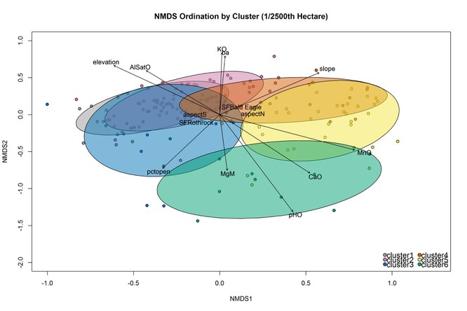
Here are some keys for interpreting the graph:
- ignore the axes – focus on the colored dots or points. Similar sampling locations are closer together on the graph.
- the colors are the groups I identified using clustering (each a different color; the ellipse includes 75% of the group’s points).
- the environmental overlay (black text and arrows) displays high values of each variable where the text is. See “slope” on the upper right side of graph? As you move along the arrow toward “slope” my sample plots are in steeper locations.
Ok, so what do you notice first? The colors? Yes!
There are 6 different “clusters”. The dark blue, gray, and pink are really similar to one another (upper left ellipses). The red and yellow groups are similar to each other, too (upper right ellipses). The green group is a loner (different from everything else).
What species make up those groups?
For the dark blue, pink, and gray clusters, it’s mostly ericaceous plants! Mountain laurel, huckleberry, and blueberry make up more than two-thirds of the vegetation in each of those clusters. The subtle differences you see between them are their relative percentages of each (84% for dark blue, 66.8% for pink, and 79.3% for gray).
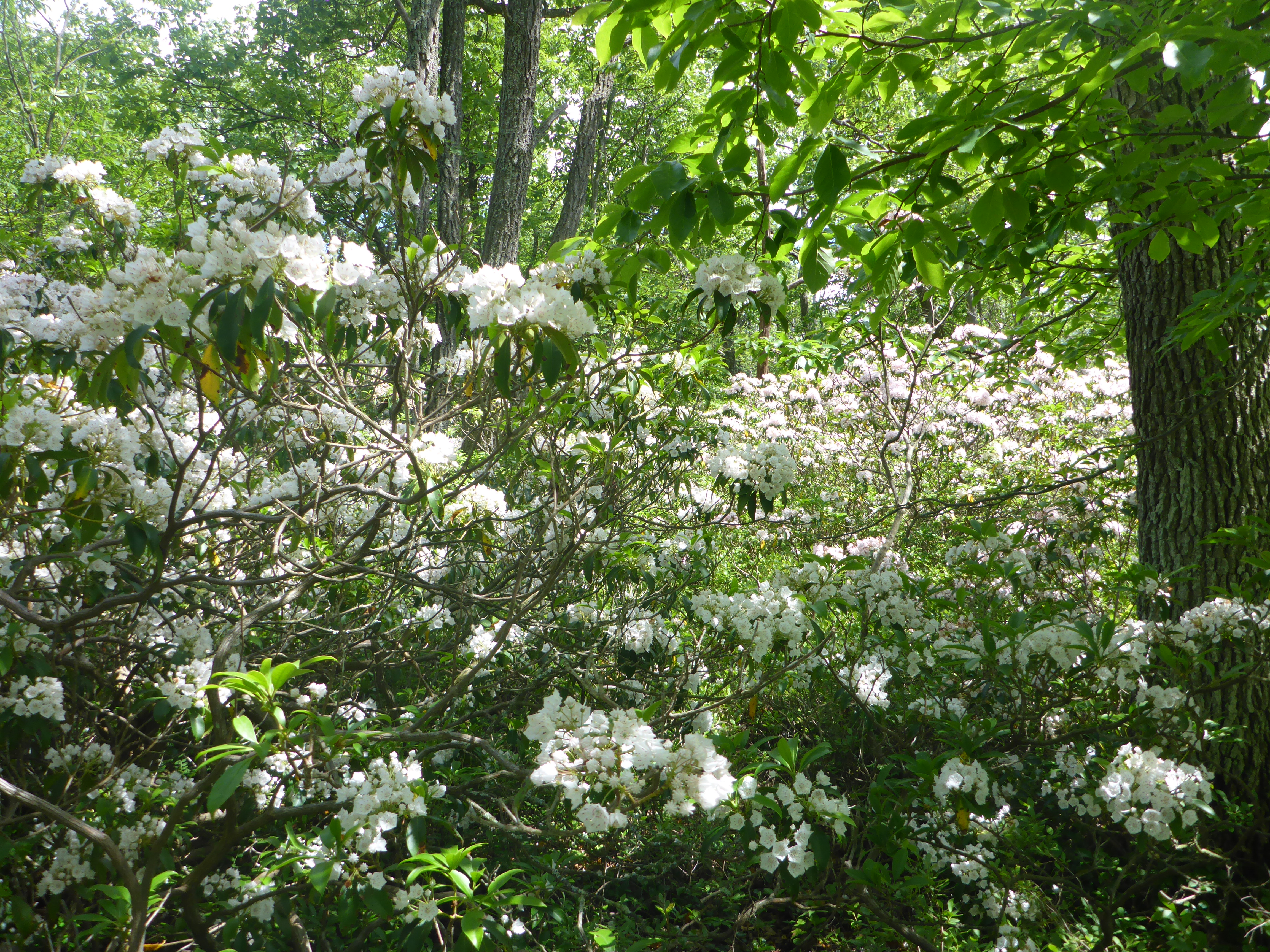
Mountain laurel is part of the ericaceous, high elevation plant community
The green cluster is comprised mostly of hay-scented fern (57.4%) and some brambles (9.7%). And, just in case you had any doubt that the ridge and valley province was a difficult place to be a plant—the red and yellow clusters are mostly rock (60.4% in red, and 31.7% in yellow) and rock-covered moss (8% red, 28.8% yellow). While there are some species that are able to grow in such an environment (appropriately called “rockfoils”) most plants don’t find rocky outcroppings a suitable place to put down roots (pun intended).
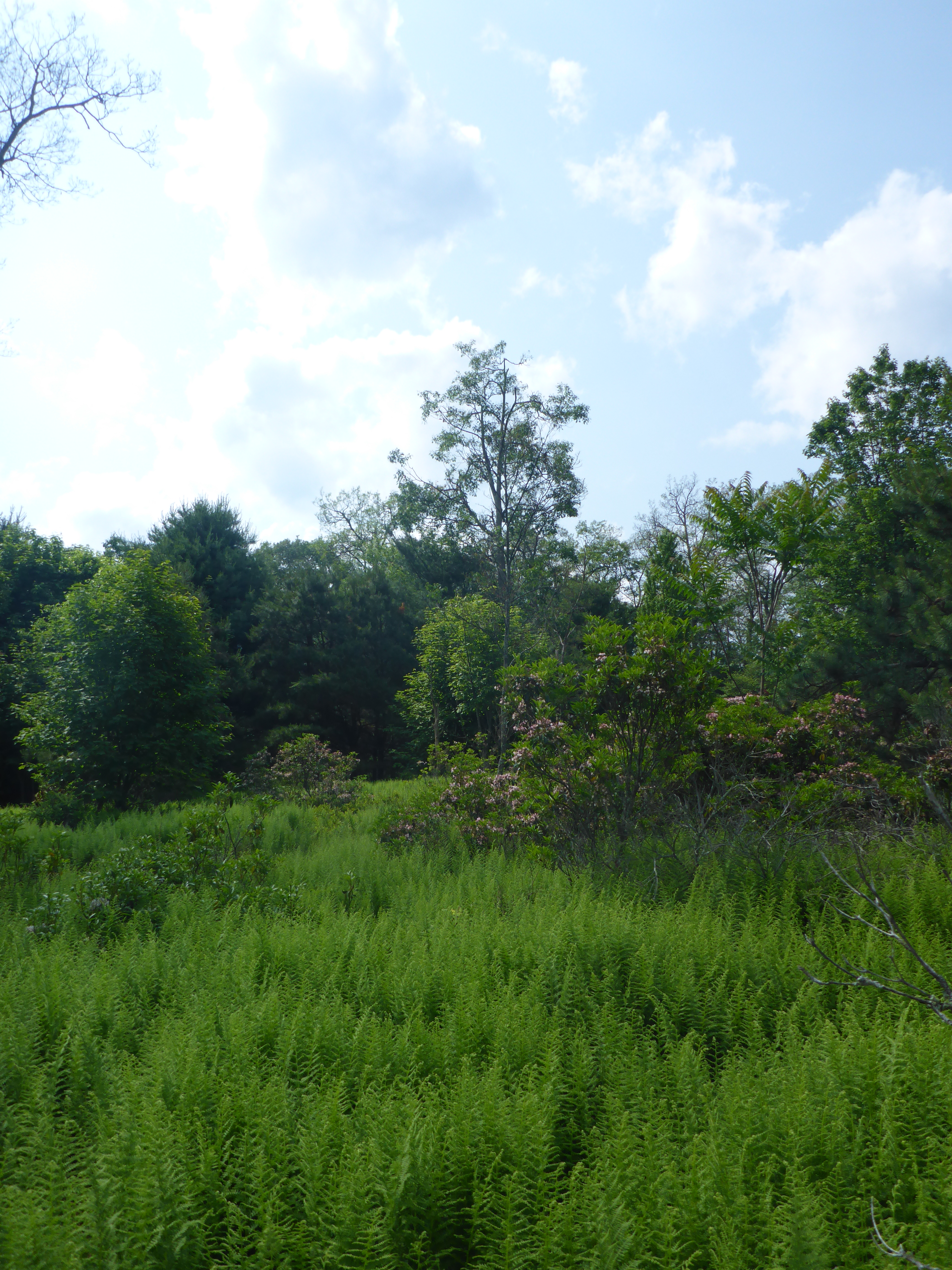
Example of a hay-scented fern dominated community
Did you notice any relationships with the environmental variables across groups?
The samples in the green cluster are associated with higher pH and higher levels of extractable Ca and Mg. They are also associated with higher levels of Mn suggesting that those hay-scented fern dominated plant communities are tolerant of higher Mn.
The rocky, red and yellow clusters have steep slopes suggesting these samples mostly fall on side slopes with poorly formed soil underneath. And the ericaceous-dominated clusters? These samples are mostly at high elevation, low pH, and high aluminum saturation suggesting that most of your ericaceous plants that dominate these groups are not sensitive to high levels of aluminum saturation in the soil. Aluminum is known to be toxic to plants, so this is a really interesting result!
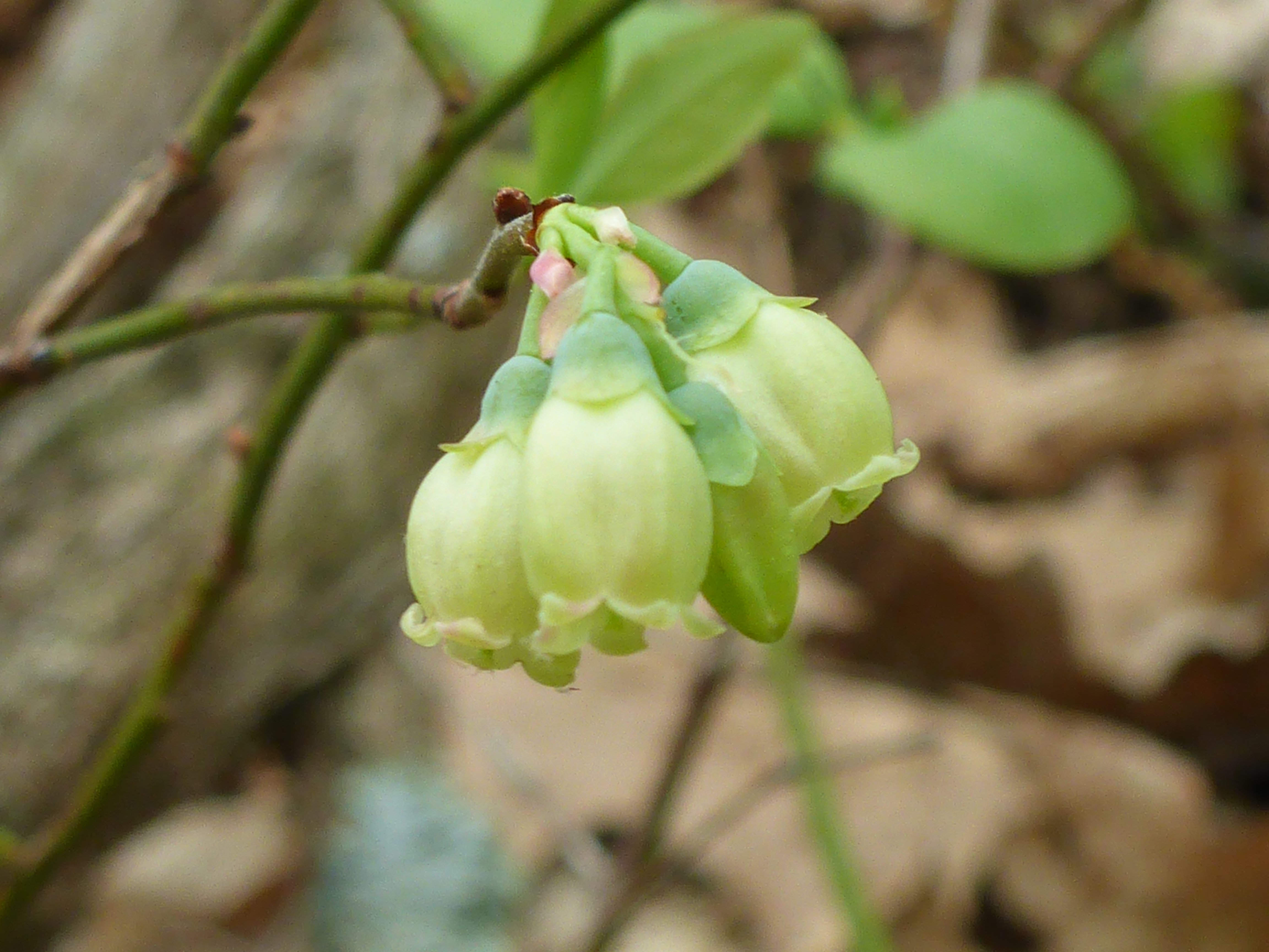
Blueberry flowers
Putting it all together, these results suggest that plant communities are responding to a variety of different environmental conditions all at once. There’s not one “smoking gun” environmental variable that explains patterns we’re seeing across the landscape. pH, Ca, Mg, Mn, Al, and elevation are all important in explaining vegetation patterns.
It’s a complicated, intertwined mess that requires multiple tests and approaches to begin to understand it. However, techniques like this provide more information than we had before, and that’s a start.
So the next time you’re out in the woods for a walk and stumble across a thick patch of mountain laurel, huckleberry, blueberry, (and maybe even some teaberry!)—it’d be a pretty good bet that you’re near the top of a ridge, walking on aluminum-saturated, low pH soil.
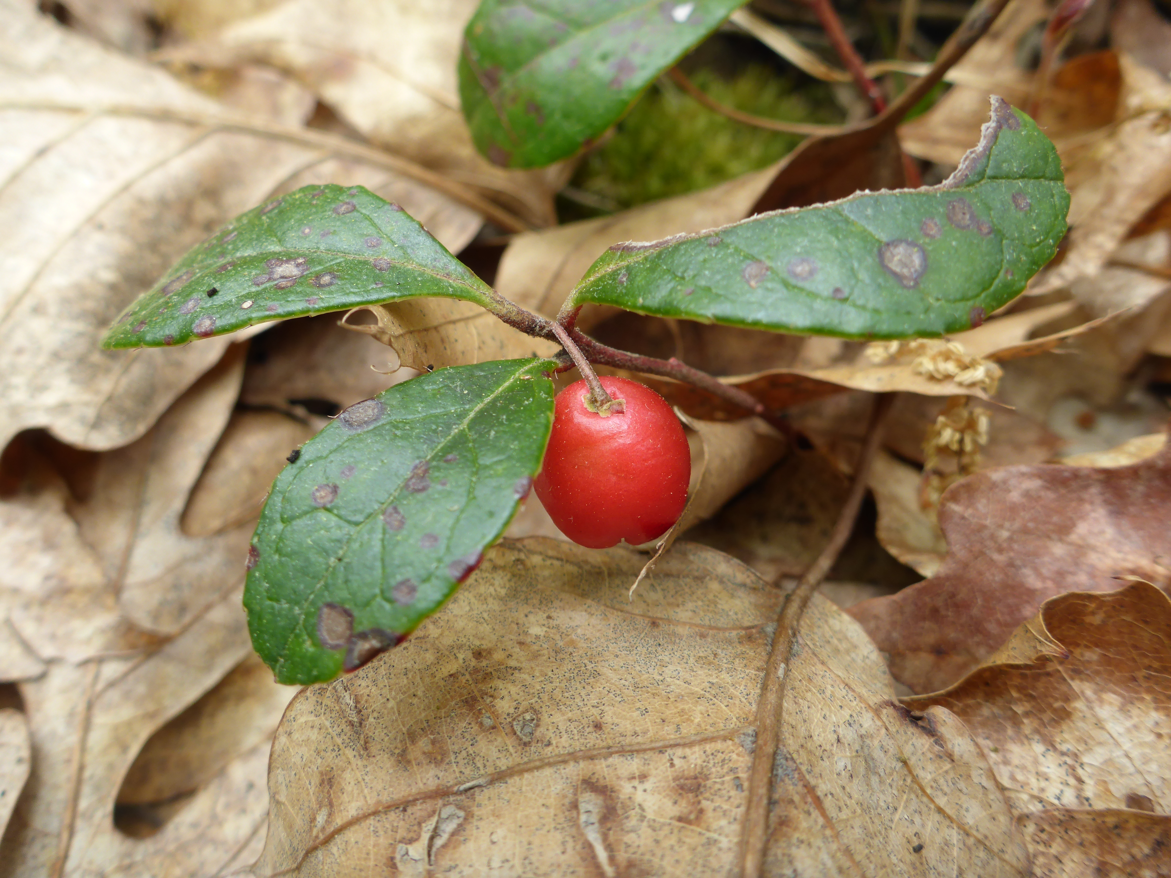
Teaberry (Gaultheria procumbens) is a diminutive plant of the understory that toleratives low light and poor soil conditions. It survives in these conditions with its evergreen leaves. The leaves and branches make a fine herbal tea and the plant is used to flavor ice cream!
Vegetation is like a book providing us a wealth of knowledge about the landscape. You just have to speak the language to read it.
Ph.D. Graduate Student